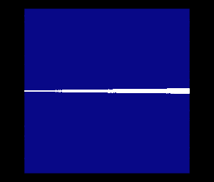

Fig 1: Narrowly bundled light streaks white cardboard from left. A glass prism refracts and reflects the beam: First at the air-glass boundary, than totally at the glass-air base and finally while exiting the prism.
Radiance is a physically based rendering package written largely by Greg Ward.
Roland Schregle added the photon-map algorithm to Radiance in his PhD at Fraunhofer ISE (download and docs at
photon-map page at FhG-ISE).
This short text describes a test with photon-maps. The test simulates a classical demonstartion setup of geometrical optics, as used
in schools.
Fig 1: Narrowly bundled light streaks white cardboard from left. A glass prism refracts and reflects the beam: First at the air-glass
boundary, than totally at the glass-air base and finally while exiting the prism.
All reflected and refracted light is modeled by photon-map. Classical Radiance would not follow reflected or refracted light-paths (Fig 2).
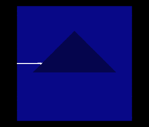
Fig 2: Classical Radiance rendering of scene in Fig 1.
void spotlight l1

0

0

7       1e9 1e9 1e9     1.5     1e-4 1e-10 0


l1 ring d1

0

0

8       -14 -0.025 0

        1 0 0

        0 1e-1
void dielectric d1

0

0

5	.9 .9 .9	1.7	0


!genprism d1 prism 3  -7 -7 0 0  7 -7   -l 0 0 2  |xform -t 0 0 -1 -rx 90 -t 0 0 5.5
void metal is

0

0

5	1 1 1	1 0
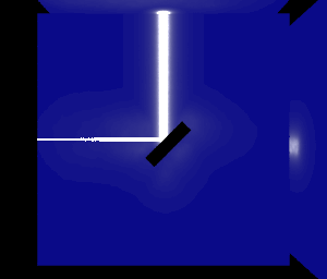
Fig 3: The reference setup (left) and a 45o inclined specular surface (right).
Additional receiving surfaces at right and top edges were added for the photon-map to work for rtrace runs (see below).
This geometry allows a first comparison between classical Radiance and photon-map: As reference rtrace is used with no optical elements to generate
irradiance values for infinitesimal surfaces at points along a line from (0.99,0,-1) to (0.99,0,+1) with surface normal (-1,0,0), along the right
edge of Fig 3 (left image). Classical rtrace in this empty scene uses "direct calculation" and serves as reference.
The photon-map-enhanced rtrace generates irradiance values for the specular box along a line from (-1,0,10) to (+1,0,10), the top edge of Fig 3.
Since the path lengths between light source and rtrace points are equal for both setups and the metal object reflects 100%, the results should
be identical.
Notes: Points for photon-map have to be coplanar with the surface, whose only purpose is to accumulate these caustic photons, whereas
standard Radiance points must not be coplanar, but rather a small distance above the surface to avoid shadowing.
To calculate rtrace values, the flat surface along the light ray direction is removed from the scene.
The word "mirror" was avoided, as this is a special radiance primitive. In fact this simple setup could be calculated using
secondary light sources and "mirror", but photon-map is more general, as will be shown in further examples.
The rtrace "red" channel is used, so the blue ambient light is not measured.
There are no global photon calculations, all irradiance values are caused by primary caustics.
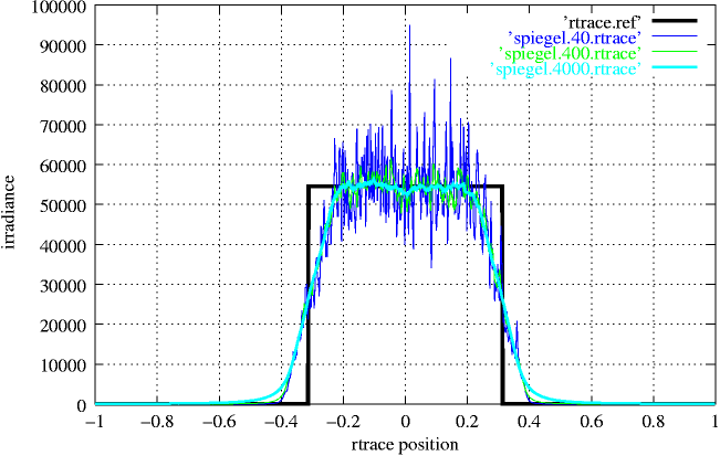
Fig 4: Irradiance for different -apc parameters. Reference curve is shown in black.
Fig4 shows irradiance results depending on the number of collected photons (-apc parameter). A total of 1 million photons had been
emitted (-apc parameter of mkpmap), and 40,400,4000 photons were collected during the rtrace run. Statistical fluctuations are
reduced by higher apc parameters, with only little bias increase at the edges. Apparently, even high apc parameters don't fully
reproduce the sharp boundaries of classical direct calculation. This might be due to Monte-Carlo (MC) sampling of Radiance's spotlight primitive.
The photon-map irradiance level match that of the direct calculations.
The small spot on the right of Fig 3 is a secondary caustic: Caustic photons bouncing of the white top wall, becoming global photons,
hitting the top edge of the box, changing to caustic photons and hitting the right wall (see Fig 5 for proof). Thanks to Roland Schregle for
pointing this out.
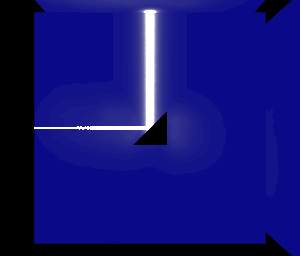
Fig 5: Reflecting prismatic box not showing secondary caustic at right wall
Fig 6: reflection off a 45o inclined surface of roughness 0.02, 0.05 and 0.1 .
This method requires slightly more descriptive details to be reproducible: Calculation of irradiance values with rtrace can be extended from sampling along a line to sampling on a regular surface grid. The photon-enhanced rtrace is fed with position vectors, e.g.:
cnt 200 200 | awk '{printf "%g %g 10 0 0 -1\n",4*(2*$1/199-1.0),4*(2*$2/199-1.0)}' | rtrace -h -oov -I -apct 0.01 -apc ... > arraydata
awk '{printf "%g\n", $4}' arraydata | pvalue -r -h -d -b -y 200 -x 200 | falsecolor -log 7 -s 1e6 ... > arraydata.pic
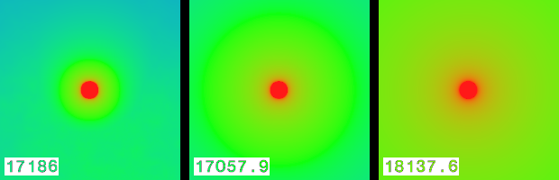
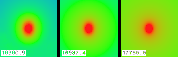
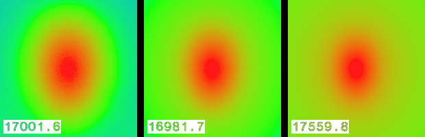
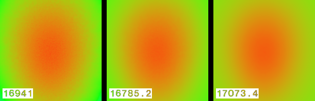
Fig 7: Irradiance levels and integrated received power at horizontal top surface of Fig 6:
logarithmic plotted rtrace data for roughness= 0.00, 0.02, 0.05, 0.10 (top down) and apc parameter of 40,400,4000 (left to right).
Fig 7 shows integrated power is within 2 percent for different roughness values, if apc 40 or 400 is used.
An expected bias for high apc values (4000) overestimates the integrated power for all roughness values.
As a check, Fig 8 shows results for a metal surface with RGB set to 0.5 (default was 1.0). Irradiance levels are scaled by 0.5, as expected.
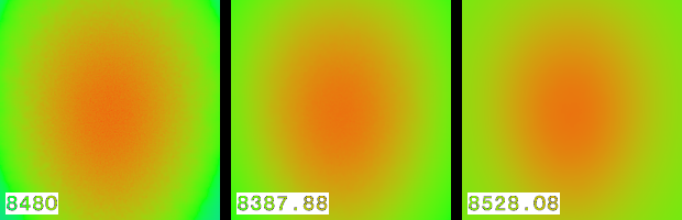
Fig 8: A cross check: setting RGB in metal surface to 0.5 with roughness 0.10
Conclusion: Photon-map with rough metal surfaces and irradiance calculations using the apc option seem to be correct in this case.
comments appreciated:
sent mail to the author
or
sent mail to the Radiance general mailing list
(remember to subscribe first, if you haven't already done so)
happy rendering,
Peter Apian-Bennewitz
software used: Radiance 3R4 with photon-map patch 3.13